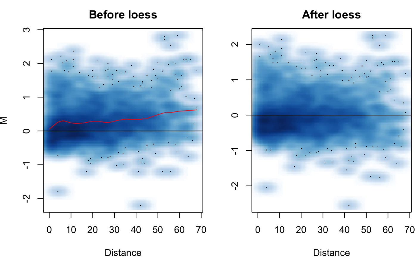
Visualize the MD plot before and after loess normalization

Visualize the MD plot before and after loess normalization

MD.plot1(M, D, mc, smooth = TRUE)

Arguments

M	The M component of the MD plot. Available from the hic.table object.
D	The D component of the MD plot. The unit distance of the interaction. Available from the hic.table object.
mc	The correction factor. Calculated by hic_loess. Available from the hic.table object after running hic_loess.
smooth	Should smooth scatter plots be used? If set to FALSE ggplot scatter plots will be used. When option is TRUE, plots generate quicker. It is recommend to use the smooth scatter plots.

Value

An MD plot.

Examples

# Create hic.table object using included Hi-C data in sparse upper
# triangular matrix format
data('HMEC.chr22')
data('NHEK.chr22')
hic.table <- create.hic.table(HMEC.chr22, NHEK.chr22, chr = 'chr22')
# Plug hic.table into hic_loess()
result <- hic_loess(hic.table)
#> Span for loess: 0.219052588777294
#> GCV for loess: 0.000118686898199309
#> AIC for loess: -0.212037314500057
MD.plot1(result$M, result$D, result$mc)