Perform joint loess normalization on two Hi-C datasets

hic_loess(
  hic.table,
  degree = 1,
  span = NA,
  loess.criterion = "gcv",
  Plot = FALSE,
  Plot.smooth = TRUE,
  parallel = FALSE,
  BP_param = bpparam()
)

Arguments

hic.table	hic.table or a list of hic.tables generated from the create.hic.table function. list of hic.tables generated from the create.hic.table function. If you want to perform normalization over multiple chromosomes from each cell line at once utilizing parallel computing enter a list of hic.tables and set parallel = TRUE.
degree	Degree of polynomial to be used for loess. Options are 0, 1, 2. The default setting is degree = 1.
span	User set span for loess. If set to NA, the span will be selected automatically using the setting of loess.criterion. Defaults to NA so that automatic span selection is performed. If you know the span, setting it manually will significantly speed up computational time.
loess.criterion	Automatic span selection criterion. Can use either 'gcv' for generalized cross-validation or 'aicc' for Akaike Information Criterion. Span selection uses a slightly modified version of the `loess.as()` function from the `fANCOVA` package. Defaults to 'gcv'.
Plot	Logical, should the MD plot showing before/after loess normalization be output? Defaults to FALSE.
Plot.smooth	Logical, defaults to TRUE indicating the MD plot will be a smooth scatter plot. Set to FALSE for a scatter plot with discrete points.
parallel	Logical, set to TRUE to utilize the `parallel` package's parallelized computing. Only works on unix operating systems. Only useful if entering a list of hic.tables. Defauts to FALSE.
BP_param	Parameters for BiocParallel. Defaults to bpparam(), see help for BiocParallel for more information http://bioconductor.org/packages/release/bioc/vignettes/BiocParallel/inst/doc/Introduction_To_BiocParallel.pdf

Value

An updated hic.table is returned with the additional columns of adj.IF1, adj.IF2 for the respective normalized IFs, an adj.M column for the adjusted M, mc for the loess correction factor, and A for the average expression value between adj.IF1 and adj.IF2.

Details

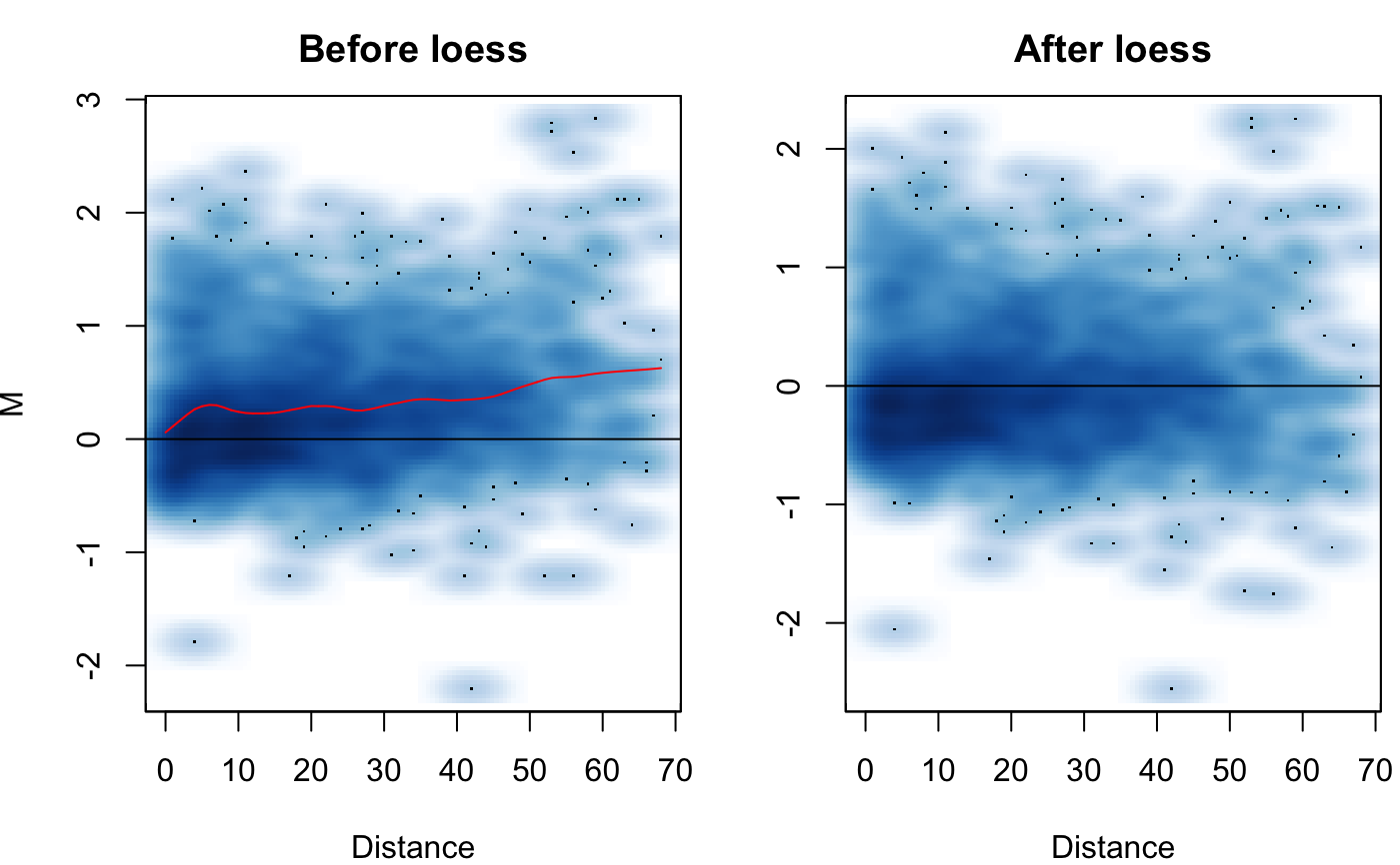
The function takes in a hic.table or a list of hic.table objects created with the create.hic.loess function. If you wish to perform joint normalization on Hi-C data for multiple chromosomes use a list of hic.tables. The process can be parallelized using the parallel setting. The data is fist transformed into what is termed an MD plot (similar to the MA plot/Bland-Altman plot). M is the log difference log2(x/y) between the two datasets. D is the unit distance in the contact matrix. The MD plot can be visualized with the Plot option. Loess regression is then performed on the MD plot to model any biases between the two Hi-C datasets. An adjusted IF is then calculated for each dataset along with an adjusted M. See methods section of Stansfield & Dozmorov 2017 for more details. Note: if you receive the warning "In simpleLoess(y, x, w, span, degree = degree, parametric = parametric, ... :pseudoinverse used..." it should not effect your results, however it can be avoided by manually setting the span to a larger value using the span option.

Examples

# Create hic.table object using included Hi-C data in sparse upper
# triangular matrix format
data("HMEC.chr22")
data("NHEK.chr22")
hic.table <- create.hic.table(HMEC.chr22, NHEK.chr22, chr= 'chr22')
# Plug hic.table into hic_loess()
result <- hic_loess(hic.table, Plot = TRUE)
#> Span for loess: 0.219052588777294
#> GCV for loess: 0.000118686898199309
#> AIC for loess: -0.212037314500057
# View result
result
#>        chr1   start1     end1  chr2   start2     end2  IF1         IF2 D
#>    1: chr22 16000000 16500000 chr22 16000000 16500000    5    5.203323 0
#>    2: chr22 16000000 16500000 chr22 16500000 17000000    2    8.672206 1
#>    3: chr22 16500000 17000000 chr22 16500000 17000000  297  480.440193 0
#>    4: chr22 16000000 16500000 chr22 17000000 17500000    5   14.742750 2
#>    5: chr22 16500000 17000000 chr22 17000000 17500000   92  277.510581 1
#>   ---                                                                   
#> 2479: chr22 49000000 49500000 chr22 51000000 51500000   21   54.634896 4
#> 2480: chr22 49500000 50000000 chr22 51000000 51500000   35   71.112086 3
#> 2481: chr22 50000000 50500000 chr22 51000000 51500000  394  339.083241 2
#> 2482: chr22 50500000 51000000 chr22 51000000 51500000 4066 2741.284207 1
#> 2483: chr22 51000000 51500000 chr22 51000000 51500000 9916 7132.021930 0
#>                 M      adj.IF1     adj.IF2        adj.M         mc           A
#>    1:  0.05750528     5.103586    5.097713 -0.001661128 0.05916641    5.100650
#>    2:  2.11639897     2.079392    8.341096  2.004074812 0.11232416    5.210244
#>    3:  0.69389392   303.153008  470.688840  0.634727512 0.05916641  386.920924
#>    4:  1.56000562     5.294664   13.922271  1.394783581 0.16522204    9.608468
#>    5:  1.59283701    95.652053  266.915059  1.480512855 0.11232416  181.283556
#>   ---                                                                         
#> 2479:  1.37943338    23.009226   49.864033  1.115787132 0.26364624   36.436630
#> 2480:  1.02273986    37.747769   65.935632  0.804666919 0.21807294   51.841701
#> 2481: -0.21655615   417.219518  320.212241 -0.381778188 0.16522204  368.715880
#> 2482: -0.56875831  4227.404883 2636.620313 -0.681082463 0.11232416 3432.012598
#> 2483: -0.47544713 10121.431725 6987.265377 -0.534613540 0.05916641 8554.348551